Variational AutoEncoder (VAE) is Easy to Understand
Before Everything
I assume you, like me, know a bit of neural networks.
I assume you, also like me, have attempted many times to understand Bayesian and have either failed or reached a state of “almost got it”.
After all, Bayesian people speak a different language from NN people, which can be counterintuitive at times. Among the hardest, there is no Andrej Karpathy yet on this topic. I am not by any measure qualified to be that guy, but only want to share what I’ve known from a rather practical point of view. By this, I mean, (and I think if there’s one thing you want to know about me this is it), I don’t think I fully understand anything before I code them up. (Of course, someone has already said that in a famous way.)
I plan to spend the time and space of 3 blog posts to make the linkage between NN and Bayesian. The current one is the first: VAE is easy to understand. Following this if you are still interested you would want to check out:
OK, let’s get started.
Variantial AntoEncoder is just a Neural Network
Most articles on VAE (including the original paper) start with posterior distribution estimation, KL divergence, variational inference, etc. Those “fancy” terms meant nothing to me at the first time. We would get lost easily if trying to understand those terms or trying to follow the equations directly. As an alternative, I prefer to start from a more practical perspective, forming an intuitive understanding of this model, how it works, and playing with the code. Then we can ask deeper questions, such as why this model works, what’s the theory behind it.
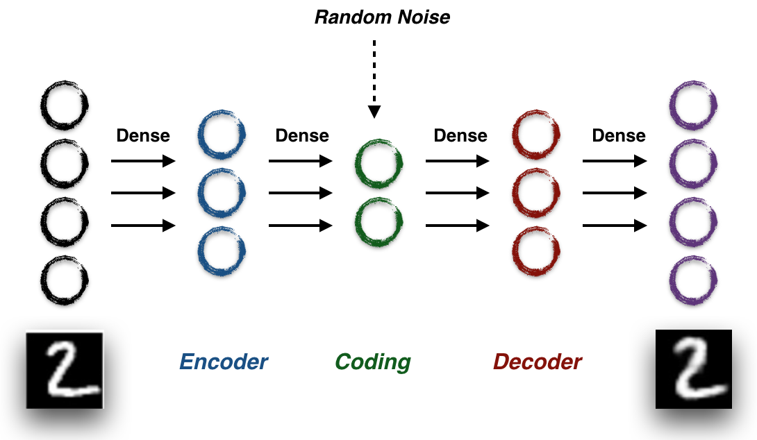
This is the structure of VAE, which is very similar to a classic AutoEncoder. We take raw image pixels as network input, going through two simple fully connected layers to project the original dimension (eg. 784 for MINST) into a lower dimension (such as 2). Then use symmetric two fully connected layers to reconstruct it back to the original image dimension. AutoEncoders, as well as VAEs, can be seen as a data compression model. In the training process, we can just set the training target as input image itself and use reconstruction error as the loss. Choosing an appropriate metric for image reconstruction is hard (but that’s another story). We’ll use the binary cross-entropy, which is commonly used for data like MNIST. Let’s visualize the structure with code (TensorFlow + Keras)
# Classic AutoEncoder
in_x = Input(shape=(784,))
encoded = Dense(128, activation='relu')(in_x)
encoded = Dense(2, activation='relu')(encoded)
decoded = Dense(128, activation='relu')(encoded)
output = Dense(784, activation='sigmoid')(encoded)
These 5 lines of code is the classic AutoEncoder. If you can train it really well, any image can be compressed into 2 numbers with the network. Then, let’s take a look at VAE.
# VAE
in_x = Input(shape=(784,))
encoded = Dense(128, activation='relu')(in_x)

z_mean = Dense(2, activation='relu')(encoded)
z_var = Dense(2, activation='relu')(encoded)
encoded = z_mean + K.exp(z_var / 2) * K.random_normal(shape=tf.shape(z_mean))

decoded = Dense(128, activation='relu')(encoded)
output = Dense(784, activation='sigmoid')(encoded)
It is almost the same as the AutoEncoder, except A) we name each of the 2 dimensions as z_mean and z_var and B) we add a random noise on the z_mean. Intuitively, this random noise serves as a ‘drop-out’-like regularizer.
Another difference between AutoEncoder and VAE is the loss function. Here is the loss of AutoEncoder, which is simply binary cross-entropy between the original image and the reconstructed.
# Classic AutoEncoder Loss
construction_loss = K.binary_crossentropy(output, in_x)
loss = tf.reduce_mean(construction_loss)
This is the VAE loss:
# VAE Loss
construction_loss = K.binary_crossentropy(output, in_x)
KL_loss = -0.5 * K.sum(1+ z_var -K.square(z_mean) - K.exp(z_var),axis=-1)

loss = tf.reduce_mean(K.mean(construct_loss, axis=-1) + KL_loss)
The only difference is VAE loss has an extra KL_loss, which is an simple function of the coding variables z_mean and z_var. We can also treat this term as a special regularizer. Notice how the word regularizer has come up a second time? Yes, VAE is just an AutoEncoder with special regularization. This regularizer provides some guidance what z_mean and z_var should look like. And because of this extra regularization term, it performs better than the classic AutoEncoder. (We will discuss why the regularizer works in later sections.)
Now, let’s have some fun training this VAE we just built, on MNIST. Firstly, let’s train this VAE with a coding dimension of 2. In another word, we are encoding a 28x28 MNIST image into 2 numbers. In this way, we can easily visualize the codes with a 2D plot.
The following figure shows the values of trained 2D coding variables of training images. Each color is a different digit class.
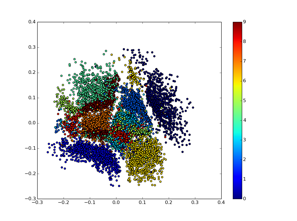
We can see different digits are well separated in the coding space already. (Bear in mind, though, this is training images.) Then let’s take a look at how well this model reconstruct our testing (unseen) images.
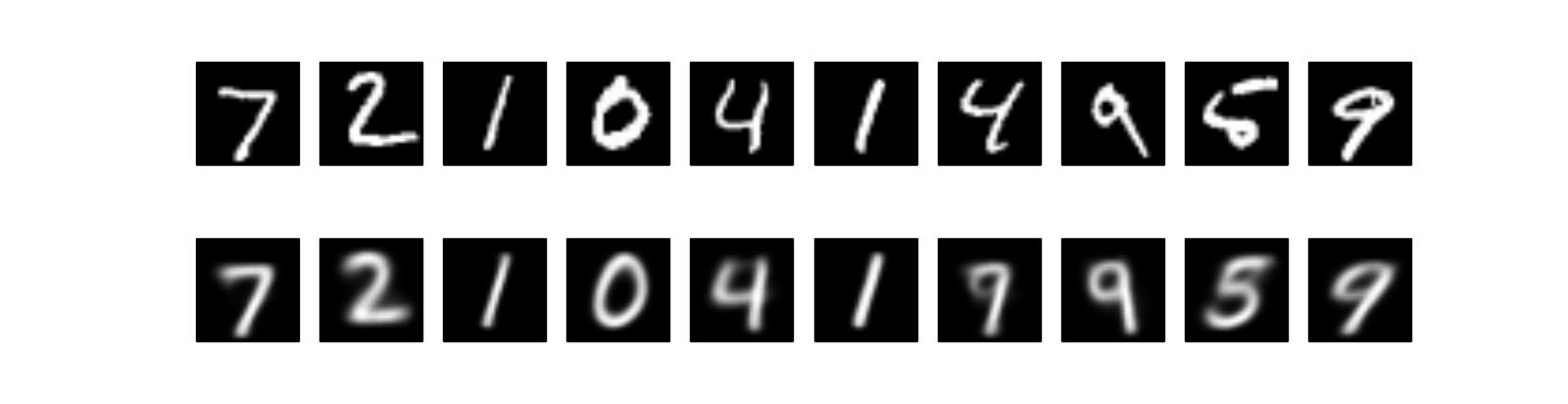
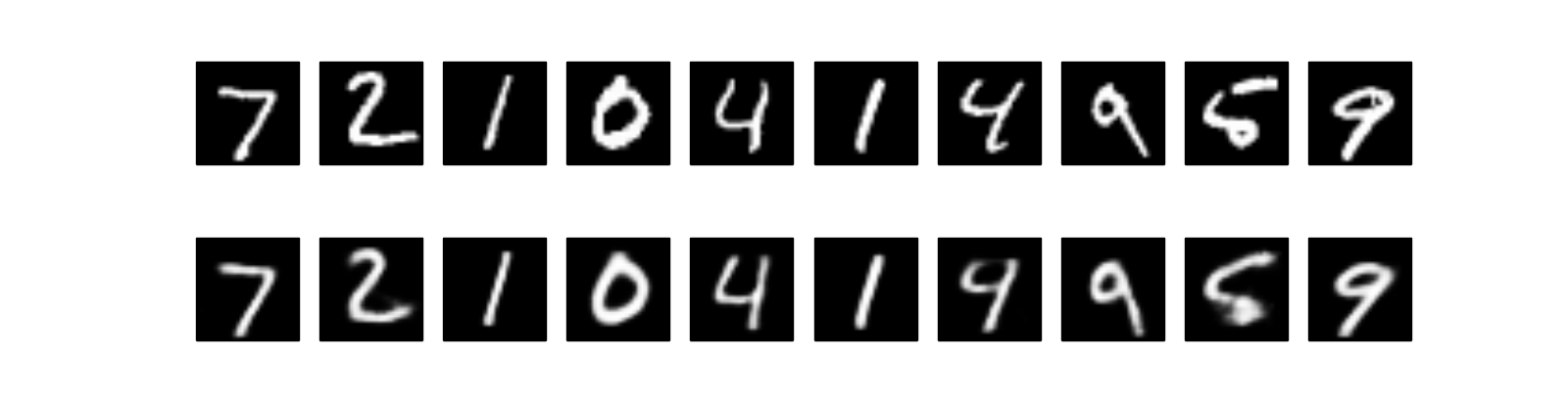
The first row is true testing images, and second row reconstructed images. It’s pretty cool, right? Even we can still see some blurring in the reconstructed images, they mostly recovered the original. Remember, we compress the \(784\) dimensions into only \(2\) dimensions! If we increase the coding dimension from \(2\) to \(12\), here are the reconstructed images. It’s much cleaner!
Also, remember VAE is a generative model, which means we can “generate” new images from nothing! Think about how we just represented a 28 x 28 image into 2 numbers. Now if we just scan the 2D space of those 2 numbers, and generate digits from there with the decoder network, here is what we see.
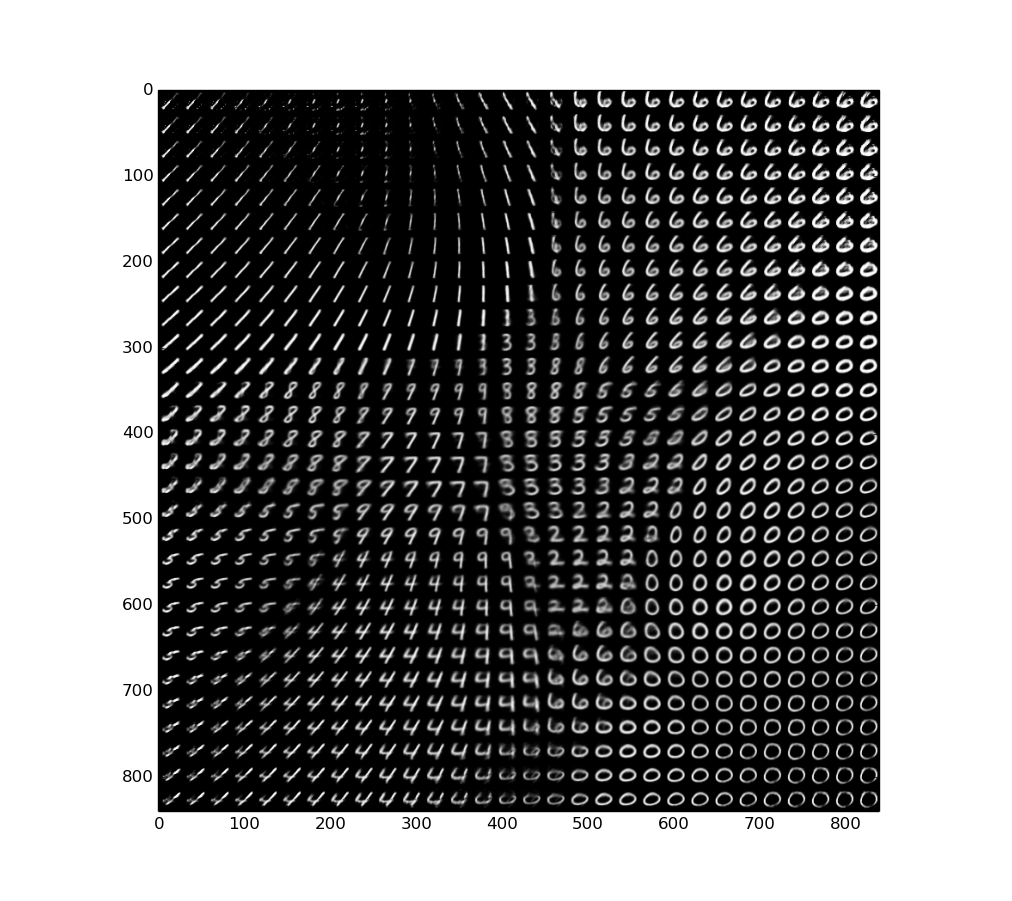
We can generate any digit from 0 to 9. If we scan from \((-0.15,-0.15)\) and slowly move those numbers to \((0.15, 0.15)\), we can see the beautiful gif of slowly emerging digits at the very top of this post.
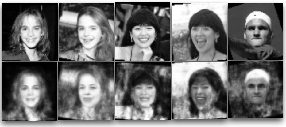
Another face image generation example (shown at the top) is trained with a latent dimension of \(200\), from this dataset. The test images displayed (of Emma Watson, Ziyi Zhang, Roger Federer) are of course not in the training set.